An Improved Retrieval Framework for Particle Size and Object-Plane Distance from Three Generations of Cloud Particle Imagers

1. INTRODUCTION

Accurate determination of cloud particle size is essential for understanding cloud microphysical processes and for interpreting observations obtained from airborne cloud probes. Over the past several decades, optical array probes (OAPs) have served as one of the primary instruments for imaging and sizing cloud particles in a wide variety of atmospheric environments. The earliest OAPs estimated particle dimensions from the number of shadowed photodiodes as particles traversed a collimated laser beam (Knollenberg, 1970). Subsequent developments introduced two-dimensional imaging capability, enabling more detailed characterization of particle geometry and morphology (Knollenberg, 1976).

The accuracy of particle sizing by OAPs has been investigated extensively. Knollenberg (1970) demonstrated that particle dimensions could be measured with an uncertainty of approximately 10% when particles remained within a specified distance of the object plane, where the optical system achieves its maximum focus. Later studies showed that the apparent particle size depends strongly on the distance between the particle and the object plane. Joe and List (1987) reported sizing errors of up to four channels for particles observed by a 2D-OAP Grey probe, particularly for particles smaller than 200 μm and for particles located farther from the object plane. Similar dependencies were also reported by Reuter and Bakan (1998), who documented increasing sizing errors with increasing object-plane displacement.

To reduce these uncertainties, two general approaches have been developed. The first approach applies statistical corrections to measured particle size spectra using empirically derived transformation matrices (Joe and List, 1987; Korolev et al., 1998; Strapp et al., 2001). The second approach attempts to reconstruct the dimensions of individual particles directly from their recorded diffraction images. Korolev et al. (1991) demonstrated that diffraction patterns generated by transparent spherical particles can be represented using Fresnel-Kirchhoff (F-K) diffraction theory for a circular disk. Building upon this framework, Korolev et al. (1998) and Korolev (2007) developed image-reconstruction methods capable of accounting for particle oversizing associated with defocused images. These studies established that particle sizing and object-plane position retrieval problems are intrinsically coupled and must be considered simultaneously.

The Cloud Particle Imager (CPI), developed by the Stratton Park Engineering Company (SPEC Inc.), provides substantially higher image resolution (2.3 μm) than conventional OAPs by recording particle diffraction images on a charge-coupled device (Lawson et al., 2001). Unlike traditional OAPs that record binary shadow information, the CPI measures grayscale 8-bit diffraction patterns containing additional information related to particle size, morphology, and image focus. Consequently, CPI observations have become widely used for investigations of ice crystal habits and cloud microphysical structure in diverse atmospheric conditions (Lawson et al., 2019).

Despite these advantages, quantitative retrieval of particle size from CPI imagery remains challenging because the apparent particle dimension depends on image focus, particle morphology, illumination conditions, and the particle position relative to the object plane. Connolly et al. (2007) developed a physically based retrieval framework that accounts for these effects using diffraction theory and an effective position parameter. Their methodology demonstrated that the particle size and object-plane distance could be estimated simultaneously from image properties extracted from CPI observations.

However, the retrieval framework of Connolly et al. (2007) was developed specifically for CPI version 1.0 and cannot be transferred directly to other CPI generations because of differences in optical alignment, illumination geometry, and image-detection characteristics (McFarquhar et al., 2013). Since multiple CPI versions have been deployed in major field campaigns and long-term observational studies (e.g., Huang et al., 2008; May et al., 2008; Vaughan et al., 2008), version-dependent retrieval biases can complicate quantitative comparison and interpretation of historical CPI datasets. A retrieval framework applicable across multiple CPI generations is therefore required to ensure consistency among observations obtained using different instrument configurations.

In this study, the original retrieval framework of Connolly et al. (2007) is revisited and extended for three generations of CPI (versions 1.0, 1.5, and 2.0). Particular emphasis is placed on retrieving the true particle maximum dimension (L) and the object-plane distance (Z) from measured image properties. A revised effective-position parameter is introduced and evaluated using laboratory observations of National Institute of Standards and Technology (NIST) calibration beads and non-spherical ice crystal analogues. Retrieval performance is assessed through comparisons between known and retrieved particle properties for each CPI version.

2. CALIBRATION METHOD

2.1 Theoretical background

When the wavelength λ of incident coherent light is significantly less than the size of an object, the F-K approximation can be used to describe the near-field diffraction patterns (Korolev et al., 1991). A schematic of F-K diffraction by a circular opaque disc is depicted in Fig. 1 with all notations summarized in Table 1.

Fig. 1.

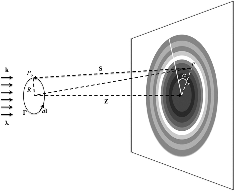
A diagram of diffraction by a circular opaque disc. All notations are summarized in Table 1. Numerical expressions of the F-K diffraction for the intensity of illumination at the P on the screen I(P) are shown in Eqs. (1)-(3).

Table 1.

Notations used to describe the diffraction by a circular opaque disc and CPI calibration.

The fundamental equations describing the diffraction by a circular opaque disc are given by

$\[ I\left(P\right)={|U^{\left(g\right)}\left(P\right)-U^{\left(d\right)}\left(P\right)|}^2, \]$

(1)

$\[ U^{\left(g\right)}\left(P\right)=\{\begin{array}{cccc}\hfill & \exp \left(ikZ\right),\hspace{0.25em}\hspace{0.25em}\hspace{0.25em}\hspace{0.25em}\hfill & \hfill & r>R\hfill \\ \hfill & 0,\hspace{0.25em}\hspace{0.25em}\hspace{0.25em}\hspace{0.25em}\hfill & \hfill & r\le R\hfill \end{array}\hspace{0.25em},\hspace{0.25em}\text{and } \]$

(2)

$\[ \begin{array}{cccc}\hfill & U^{\left(d\right)}\left(P\right)\hfill & \hfill & =\frac{1}{4𝜋}{\text{∮}}_{\mathrm{\Gamma }}\frac{\exp \left(ikS\right)}{S}\frac{\cos (n,S)}{1+\cos (S,Z)}\sin (Z,dl)dl\hfill \\ \hfill & \hfill & \hfill & =-\frac{1}{4𝜋}{\int }_0^{2𝜋} \frac{\exp \left(ikS\right)[R^2-Rr\cos \left(𝛼\right)]}{S(S-Z)}d𝛼\hfill \end{array} \]$

(3)

where n is a unit vector normal to the direction of propagation of the incident wave, and dl is a differential line element along the boundary Γ. Equation (1) expresses the screen intensity I(P) as the squared magnitude of the difference between the geometrical-optics field, U^(g)(P), and the boundary-diffraction field, U^(d)(P). In Eq. (2), U^(g)(P) = 0 inside the geometrical shadow (r ≤ R), whereas U^(g)(P) = exp(ikZ) outside the shadow (r > R). Equation (3) represents the diffraction contribution as a boundary integral over Γ (Born and Wolf, 1999). According to Babinet’s principle, the diffraction fields produced by a circular opaque disc and a circular aperture differ only in sign. Equations (1)-(3) constitute the Rubinowicz representations of the Kirchhoff diffraction integral and provide a mathematical formulation of Young’s boundary-diffraction theory. Further details are provided by Korolev et al. (1991), Korolev et al. (1998), and Connolly et al. (2007).

The apparent particle size measured by OAPs increases with the absolute distance of the particle from the object plane, resulting in distance-dependent particle oversizing (Korolev et al., 1991; Baumgardner and Korolev, 1997; Korolev et al., 1998; Strapp et al., 2001). The reduction in image quality with distance from the object plane defines the depth of field (DOF). For example, it was shown that a threshold of 40% of the laser intensity in OAPs defines the distance along the laser beam within which all recognizable images originate and the sizes of all particle images differ from the true particle sizes by less than about 10%, and this distance was called the “DOF” (Knollenberg, 1970). The F-K diffraction reveals that the diffraction images can be represented in terms of their normalized position Z_d = λ|Z|/R², and are not dependent on the sign of Z (Korolev et al., 1998). Based on these findings and the F-K diffraction theory, an OAPs correction algorithm for reconstructing true size of particles was developed by Korolev et al. (1998).

3. LABORATORY CALIBRATION PROCEDURE AND CALIBRATION EQUATIONS

A fundamental problem associated with both OAPs and CPIs is that the apparent maximum dimension L_app of a particle extracted from an image differs from its actual maximum dimension L. Past studies have shown that the particle oversize L_app/L can be quantified as a function of certain variables, such as Z_d. Thus, the CPI calibration procedure involves finding the principal variables and optimal calibration equations that govern oversize L_app/L.

3.1 Laboratory calibration procedure

The purpose of the laboratory calibration procedure is to generate images of particles that resemble realistic cloud particles. Unlike data obtained during aircraft flights through cloud, laboratory images of cloud particles can be used to determine the calibration because both the size (L) and position (Z) of the particles are known and can be controlled. Repeated measurements for the same particles at varying Z are also possible in the laboratory. Thus, the dependence of oversize L_app/L on independent variables and the corresponding calibration equations can be determined.

The National Institute of Standards and Technology certified spherical glass calibration beads and novel non-spherical ice crystal analogues (Ulanowski et al., 2003; Ulanowski et al., 2006) were used in the calibration procedure. The ice-crystal analogues are sodium fluorosilicate (Na₂SiF₆) crystals grown from solution on glass substrates and exhibit morphologies and optical properties similar to those of idealized atmospheric ice-crystal habits. In this study, 6 different sizes of spherical glass beads and 9 different shapes and sizes of ice analogues were used (Table 2). Example images of the ice analogues are shown in Fig. 7 of Connolly et al. (2007).

Table 2.

Sizes of glass beads and ice analogues used in the calibration procedure.

For the procedure, the glass calibration beads or the ice analogues were first placed on a glass slide mounted on a calibration rig (left panel of Fig. 2). The rig was then inserted into the outer inlet of the CPI (right panel of Fig. 2). The glass slide was positioned at 45^o to the axis of the CPI sample tube so that all particles on the glass slide were equidistant from the object plane of the CPI. This 45^o position placed the glass slide perpendicular to the imaging laser because the imaging laser is positioned at 45^o to the axis of the CPI sample tube as shown in Fig. 3. The glass slide was moved from one side of the DOF, through the position of the object plane, to the other side of DOF (i.e., out of focus to good focus and then out of focus) in regular increments as measured by three micrometer gauges attached to the calibration rig (Fig. 2). The glass slide was assumed to be at the position of the object plane when the maximum focus value was measured by the CPI controlling software. The absolute distance Z between a particle and the object plane was then calculated from the position by a coordinate transformation of 45^o in the x-z plane (See Fig. 3).

Fig. 2.

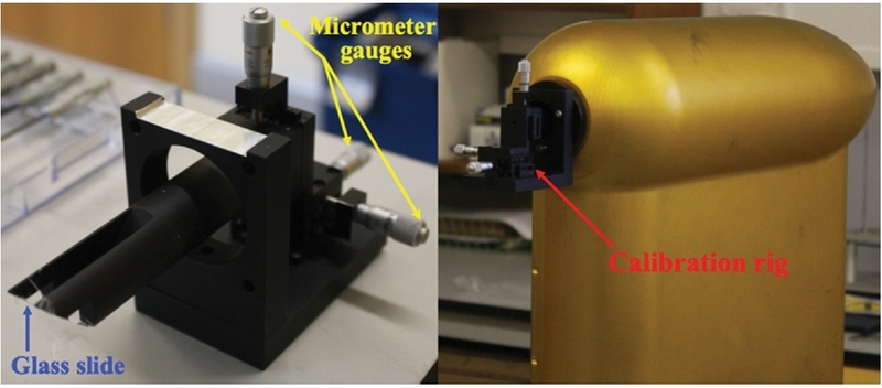
Photographs of the laboratory calibration setup. (Left) The calibration rig equipped with a glass slide and micrometer gauges. (Right) The rig mounted on the CPI during calibration.

Fig. 3.

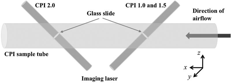
Difference in the position of imaging laser in CPI 2.0 (left) and CPI 1.0 and 1.5 (right). During the calibration procedure, either glass calibration beads or ice analogues were placed on the glass slide shown in the middle of each imaging laser. The calibration rig housing the glass slide is not shown. The direction of airflow is indicated by the thick arrow. The coordinate system used to calculate the position of the glass slide is embedded.

Since the optical system and external shape of the CPI version 2.0 differ from those of the earlier versions 1.0 and 1.5, some modifications to the original calibration rig used by Connolly et al. (2007) were necessary. The object plane of CPI version 2.0 is rotated by 90^o relative to those of the earlier versions. (See Fig. 3). Accordingly, the part of the calibration rig that houses the glass slide was rotated 180^o to ensure that all particles were an equal distance from the object plane. In addition, the coordinate transformation needed to calculate the distance between the particle and object plane for CPI version 2.0 was adjusted.

The procedure of moving the glass slide from one side of the DOF to the other was repeated for the glass calibration beads and ice analogues of varying sizes. The distance (Z) between each particle and the object plane was calculated by the coordinate transformation, and the relative illumination (i.e., $$ B{G}_{loc}/\stackrel{-}{BG}$$) was obtained from custom-written software. The CPIview software then extracted particle information (i.e., L_app, A_r, and focus) from each image.

3.2 Calibration equations

Korolev et al. (1998) showed that spherical particle oversizing observed by OAPs can be represented in terms of the normalized position Z_d. By ignoring the term for the constant λ and replacing R with L, Z_d is written as Z_d = Z/L². Figure 4 shows the particle oversize L_app/L as a function of Z_d. The L_app/L changes faster on the negative side of the object plane (i.e. for Z < 0), which corresponds to the side closer to the CPI imaging laser. Furthermore, the Korolev et al. (1998) Z_d formulation was found to systematically underestimate particle oversizing in CPI observations, particularly for particles with low A_r values (e.g., non-spherical particles; Connolly et al., 2007). These results indicate that Z_d, which is independent of the sign of particle displacement, does not adequately represent particle oversizing observed by the CPI.

Fig. 4.

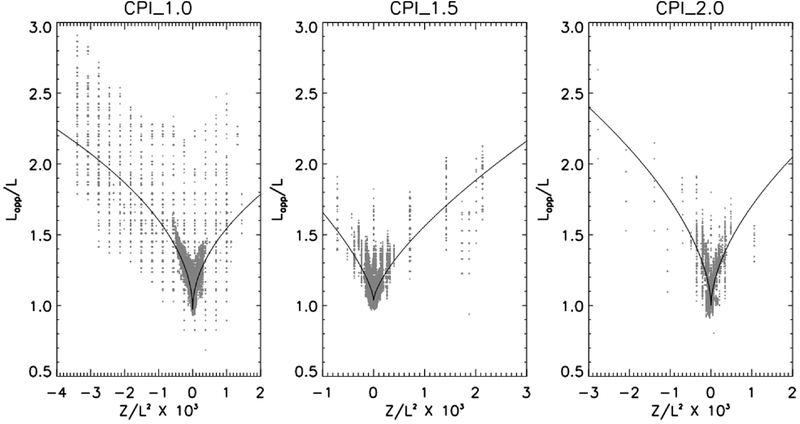
Particle oversize (Lapp/L) by CPI 1.0 (left), 1.5 (middle), and 2.0 (right) as a function of Z/L2. The best-fit curve, Lapp/L = a1 × (|Z/L2| + Z/L2)a2, where a1 and a2 are constant, is shown in each panel.

Connolly et al. (2007) introduced a new empirical quantity, an effective position Z_eff = Z/(LA_r)², to better quantify the oversizing L_app/L induced by a CPI 1.0. By examining the calibration data collected for the three CPIs here, it was seen that a slightly different expression for Z_eff, namely Z_eff = Z/(L²A_r), gave smaller residual errors than the original expression when representing the oversize L_app/L measured by a CPI. To distinguish between the two formulations, the original and revised effective-position parameters are hereafter denoted as Z_{eff_old} = Z/(LA_r)² and Z_{eff_new} = Z/(L²A_r), respectively. Figure 5 shows L_app/L as a function of Z_{eff_new}. The change in L_app/L is asymmetrical with Z_{eff_new} in that it changes at a faster rate on the negative side of the object plane (i.e., Z < 0). Since Ar is defined as the ratio of the particle-projected area to the area of a circle with a diameter of L, Z_d, Z_{eff_old}, and Z_{eff_new} are identical for spherical particles (i.e., A_r = 1) except for the sign difference when Z < 0. However, Z_{eff_old} is largest and Z_d smallest for a non-spherical particle (A_r < 1) for a given Z and L. This causes an underestimation of particle oversize expressed with Z_d for particles with low A_r as reported in Connolly et al. (2007). These results demonstrate that Z_d does not adequately characterize particle oversizing in CPI observations, particularly for particles with low A_r. Consequently, incorporation of particle morphology through the revised effective-position parameter provides a more appropriate basis for CPI calibration.

Fig. 5.

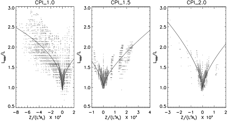
Particle oversize (Lapp/L) by CPI 1.0 (left), 1.5 (middle), and 2.0 (right) as a function of Zeff_new = Z/(L2Ar). A best-fit curve, Lapp/L = a1 × (|Z/(L2Ar)| + Z/(L2Ar))a2, where a1 and a2 are constant, is shown in each panel.

In addition to depending on Z_{eff_new}, L_app/L also decreases with increasing particle size L. This indicates that errors in the sizing of particles by CPIs are larger for smaller particles because of the larger uncertainty associated with the number of shadowed pixels. Equation (4) parameterizes the particle-oversizing L_app/L, as a function of object-plane displacement, particle morphology, background illumination, and particle size.

$\[ \frac{L_{app}}{L}=d_1\times {(\left|\frac{Z}{L^2{A}_r}\right|+d_2\frac{Z}{L^2{A}_r})}^{d_3}\times \left(\frac{B{G}_{loc}}{\stackrel{-}{BG}}\right)+d_4\times {\left(L\right)}^{d_5}, \]$

(4)

where d_n (n = 1, …, 5) are calibration parameters that are determined by the nonlinear least-squares minimization method described in the next section.

L_app, A_r, and $$ B{G}_{loc}/\stackrel{-}{BG}$$ in Eq. (4) are extracted from an in-situ particle image as previously discussed. Two unknowns (L and Z) remain and, therefore, one more equation is necessary to calculate L_app/L. Connolly et al. (2007) showed that the focus value (foc, the gradient of the image intensity at the particle edge) depends on Z. The measured foc can thus be used to calculate Z, which can then be used in Eq. (4) to determine the particle oversizing.

Figures 6 and 7 show CPI images of 60 μm beads and plate ice analogues with L = 102 μm, respectively, at varying distances (Z) from the object plane. As the absolute value of Z increases, the quality of the images decreases, the foc value decreases, and the particle oversize L_app/L increases. A relationship between foc and Z with a corresponding best-fit curve determined by minimizing residual errors is shown in Fig. 8. The large spread of foc for a given Z occurs because the detected edge of a particle depends on the relative illumination ($$ B{G}_{loc}/\stackrel{-}{BG}$$).

Fig. 6.

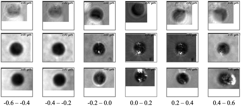
Example CPI images of 60 μm beads taken by CPI 1.0 (top row), 1.5 (middle row), and 2.0 (bottom row) as a function of distance (Z) from the object plane. The numbers at the bottom of each column indicate Z relative to the object plane (mm).

Fig. 7.

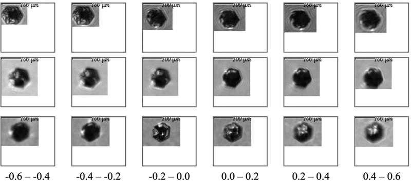
Same as Fig. 6, but for a plate analogue with maximum dimension (L) of 102 μm.

Fig. 8.

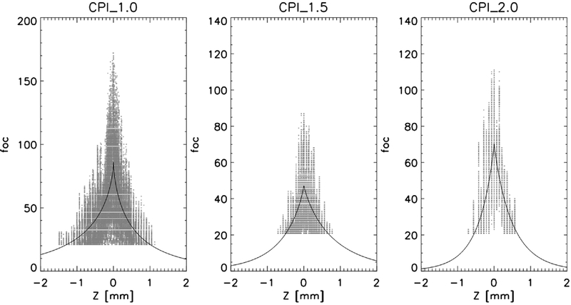
The focus value (foc) of three CPIs (left: CPI 1.0, middle: CPI 1.5, and right: CPI 2.0) as a function of Z. A best-fit curve, foc = a1 × EXP(−a2 × |Z + a3|Z||a4), where a1, a2, a3, and a4 are constant, is embedded in each panel.

Due to the resolution (2.3 µm) of a CPI, the detection of particle edge and hence the foc becomes worse for smaller particles. The roundness (A_r) of a particle also affects the foc. For example, the foc decreases with a decrease of A_r because the foc is calculated based on the shortest dimension of the particle rather than the longest dimension L (Connolly et al., 2007). Equation (5) relates the image-focus metric foc to the object-plane distance Z, while accounting for the effects of particle size, roundness, and background illumination.

$\[ \begin{array}{cccc}\hfill & foc=\hfill & \hfill & \left|c_1\right|\times {\left(\frac{B{G}_{loc}}{\stackrel{-}{BG}}\right)}^{c_2}\times {\left(L\right)}^{c_3}\times {\left(A_r\right)}^{c_4}\hfill \\ \hfill & \hfill & \hfill & \times EXP(-\left|c_5\right|\times |Z+c_6|Z{\Vert }^{\left|c_7\right|})\hfill \end{array} \]$

(5)

where c_n (n = 1, ..., 7) are calibration parameters to be determined in next section. Because L and Z are unknown, Eqs. (4) and (5) are solved simultaneously using nonlinear least-squares minimization to retrieve both quantities from the measured image properties.

In the calibration equations [Eqs. (4) and (5)], the foc, A_r, and L_app are known from the CPIview image processing software and $$ B{G}_{loc}/\stackrel{-}{BG}$$ is calculated from custom-written software (Connolly et al., 2007). Because Eqs. (4) and (5) represent two equations with two unknowns (i.e., L and Z), they can be solved iteratively using a non-linear least squares minimization method (e.g., the Levenberg-Marquardt method). However, in order to use these equations, the calibration parameters (c₁ through c₇ and d₁ through d₅) must first be determined using a laboratory calibration procedure. The calibration procedure involves imaging glass calibration beads and ice analogues of known size (i.e., L) at varying positions across the sample volume (i.e., from which Z is determined). The unknown calibration parameters are then determined by minimizing the sum of the squares of the residuals of the equations using the large calibration datasets. After deriving the calibration parameters, Eqs. (4) and (5) can be applied to calculate Z and L from in-situ field observations.

4. RESULTS

The calibration parameters derived for CPI versions 1.0, 1.5, and 2.0 are summarized in Table 3. Differences among the parameter sets reflect variations in optical alignment and image-detection characteristics across the three CPI generations. Using these version-specific calibration coefficients, Eqs. (4) and (5) can be iteratively solved to retrieve the true particle maximum dimension (L) and object-plane distance (Z) from the measured image properties. The performance of the retrieval framework is evaluated by comparing the retrieved particle properties with the known sizes and positions of the calibration beads and ice analogues in this section.

Table 3.

Calculated coefficients for Eqs. (4) and (5) derived from the laboratory calibration procedure.

Figure 9 shows the effect of applying the calibration on particle oversize (L_app − L)/L determined from the different versions of CPI. The average errors in sizing particles by the CPI 1.0 (1.5 and 2.0) before calibration (left column) were 16.1% (13.4% and 13.5%), respectively. CPI version 1.0 exhibited the largest spread in particle oversizing before the calibration. However, this spread and the larger particle-oversizing errors do not imply the performance of the CPI 1.0 was worse than the other two CPIs. Rather, it reflects the larger number of CPI 1.0 calibration particles located farther from the object plane, as shown in Fig. 10. After the calibration is applied (right column of Fig. 9), the average error in sizing particles was reduced to 5.1% (5.2% and 4.9%) for the CPI 1.0 (1.5 and 2.0), respectively. The standard deviations in the particle oversizing were also reduced when the calibration was applied.

Fig. 9.

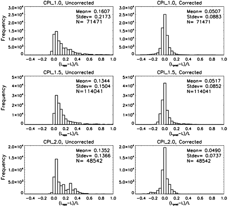
Histograms of uncorrected (left column) and corrected (right column) oversize (Lapp − L)/L of beads and ice analogues by CPI 1.0 (top row), 1.5 (middle row), and 2.0 (bottom row). The mean, standard deviation, and total number of particles are embedded in each panel. For calculation of mean values, the absolute values of (Lapp − L)/L are averaged.

Fig. 10.

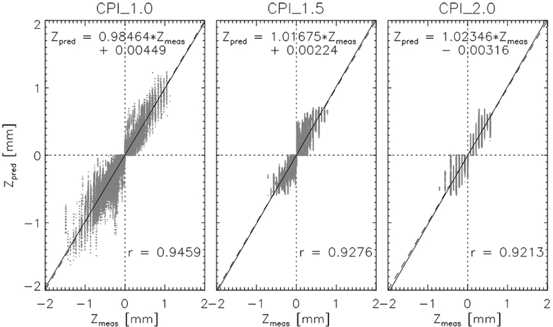
The measured Z (Zmeas) vs. predicted Z (Zpred) from the object plane of CPI 1.0 (left), 1.5 (middle), and 2.0 (right). The dashed line indicates the one-to-one relationship, whereas the solid line represents the linear regression fit shown at the top of each panel. A correlation (Pearson’s r) is also embedded in each panel.

When errors in sizing particles are corrected through application of the calibration, the Z is also corrected. Figure 10 shows the relationship between the measured Z (Z_meas) and the predicted Z (Z_pred) for the beads and ice analogues used in the calibration procedure. The Z_meas is measured during the calibration procedure, while the Z_pred is calculated from calibration equations [Eqs. (4) and (5)]. For each version of the CPI Z_pred and Z_meas are highly correlated.

In summary, application of the calibration reduced both the average sizing errors and the standard deviations for all three CPI versions. Further, Z_pred has a strong one-to-one relationship with Z_meas with high positive correlation. This indicates that the calibration given by Eqs. (4) and (5) accurately reproduces the measured particle properties.

5. SUMMARY AND DISCUSSION

A retrieval framework for estimating the maximum dimension (L) of a two-dimensional particle image and object-plane distance (Z) from CPI observations was developed and evaluated for three generations of CPI (versions 1.0, 1.5, and 2.0). The framework extends the calibration methodology originally proposed by Connolly et al. (2007) and incorporates a revised effective-position parameter, Z_{eff_new} = Z/(L²A_r), to improve representation of particle oversizing associated with defocused particle images.

Laboratory calibration experiments were performed using NIST-certified glass calibration beads and non-spherical ice crystal analogues of known size and position. The calibration datasets were used to determine version-specific coefficients for the particle-sizing and focus equations. These coefficients were subsequently applied to retrieve L and Z through iterative solution of Eqs. (4) and (5).

Application of the retrieval framework substantially reduced sizing uncertainties for all three CPI versions. Average sizing errors were reduced from 16.1%, 13.4%, and 13.5% before calibration to 5.1%, 5.2%, and 4.9% after calibration for CPI 1.0, 1.5, and 2.0, respectively. In addition, retrieved object-plane distances (Z) showed strong agreement with independently measured values, with correlation coefficients exceeding 0.92 for all CPI versions. These results demonstrate that the retrieval framework successfully accounts for differences in optical alignment and image-detection characteristics among the three CPI generations.

The results also indicate that the revised effective-position parameter provides a more appropriate representation of CPI image oversizing than the original formulation. Unlike OAP-based sizing corrections that primarily depend on normalized distance, particle sizing by a CPI is influenced by the combined effects of particle size, particle morphology, image focus, and background illumination. Incorporating these factors within a unified retrieval framework improves the consistency of particle sizing across different CPI generations.

The scope of this study is intentionally limited to the retrieval of particle size and object-plane distance from CPI imagery. Derivation of depth of field, sample volume, particle concentration, and particle size distributions was not considered. These quantities depend directly on the accuracy of retrieved particle size and position and therefore require additional evaluation. Future work should investigate how the retrieval framework developed in this study influences depth-of-field determination, sample-volume estimation, and ultimately particle concentration and particle size distribution measurements.

Overall, the retrieval framework developed here provides a consistent methodology for reducing sizing uncertainties and harmonizing observations obtained from different generations of the CPI. The results provide a foundation for future quantitative analyses of historical CPI datasets and for improving the consistency of cloud particle measurements obtained using multiple CPI versions. The calibration framework presented here may also be applicable to newer CPI generations, provided that version-specific calibration coefficients are determined through the laboratory procedure described in this study. For example, the CPI version 2.5 currently operated in the Korea Cloud Physics Experimental Chamber (K-CPEC; Park et al., 2025) could be calibrated using the same methodology. However, the calibration coefficients reported in this study should not be directly applied because of differences in instrument configuration.

Acknowledgments

This work was supported by a 2-Year Research Grant of Pusan National University. The authors gratefully acknowledge Dr. C. Emersic and Dr. Z. Ulanowski for their contributions to the calibration experiments.

References

• Baumgardner, D., and A. Korolev, 1997: Airspeed corrections corrections for optical array probe sample volumes. J. Atmos. Oceanic Technol., 14, 1224-1229. [https://doi.org/10.1175/1520-0426(1997)014<1224:ACFOAP>2.0.CO;2]
• Born, M., and E. Wolf, 1999: Principles of Optics: Electro-magnetic Theory of Propagation, Interference and Diffraction of Light. 7th ed. Cambridge University Press, 952 pp.
• Connolly, P. J., M. J. Flynn, Z. Ulanowski, T. W. Choularton, M. W. Gallagher, and K. N. Bower, 2007: Calibration of the cloud particle imager probes using calibration beads and ice crystal analogs: The depth of field. J. Atmos. Oceanic Technol., 24, 1860-1879. [https://doi.org/10.1175/JTECH2096.1]
• Huang, Y., and Coauthors, 2008: The development of ice in a cumulus cloud over southwest England. New J. Phys., 10, 105021. [https://doi.org/10.1088/1367-2630/10/10/105021]
• Joe, P., and R. List, 1987: Testing and performance of two-dimensional optical array spectrometers with grey-scale. J. Atmos. Oceanic Technol., 4, 139-150. [https://doi.org/10.1175/1520-0426(1987)004<0139:TAPOTD>2.0.CO;2]
• Knollenberg, R. G., 1970: The optical array: An alternative to scattering or extinction for airborne particle size determination. J. Appl. Meteorol., 9, 86-103. [https://doi.org/10.1175/1520-0450(1970)009<0086:TOAAAT>2.0.CO;2]
• Knollenberg, R. G., 1976: Three new instruments for cloud physics measurement: the 2-D spectrometer, the forward scattering spectrometer probe and the active scattering aerosol spectrometer. Preprints Int. Conf. on Cloud Physics. Boulder, 544-561.
• Korolev, A., 2007: Reconstruction of the sizes of spherical particles from their shadow images. Part I: Theoretical considerations. J. Atmos. Oceanic Technol., 24, 376-389. [https://doi.org/10.1175/JTECH1980.1]
• Korolev, A., J. W. Strapp, and G. A. Isaac, 1998: Evaluation of the accuracy of PMS optical array probes. J. Atmos. Oceanic Technol., 15, 708-720. [https://doi.org/10.1175/1520-0426(1998)015<0708:EOTAOP>2.0.CO;2]
• Korolev, A., S. V. Kuznetsov, Y. E. Makarov, and V. S. Novikov, 1991: Evaluation of measurements of particle size and sample area from optical array probes. J. Atmos. Oceanic Technol., 8, 514-522. [https://doi.org/10.1175/1520-0426(1991)008<0514:EOMOPS>2.0.CO;2]
• Lawson, R. P., B. A. Baker, C. G. Schmitt, and T. L. Jensen, 2001: An overview of microphysical properties of Arctic clouds observed in May and July 1998 during FIRE ACE. J. Geophys. Res. Atmos., 106, 14989-15014. [https://doi.org/10.1029/2000JD900789]
• Lawson, R. P., and Coauthors, 2019: A review of ice particle shapes in cirrus formed in situ and in anvils. J. Geophys. Res., 124, 10049-10090. [https://doi.org/10.1029/2018JD030122]
• May, P. T., J. H. Mather, G. Vaughan, C. Jakob, G. M. McFarquhar, K. N. Bower, and G. G. Mace, 2008: The tropical warm pool international cloud experiment. Bull. Amer. Meteor. Soc., 89, 629-646. [https://doi.org/10.1175/BAMS-89-5-629]
• McFarquhar, G. M. , J. Um, and R. Jackson, 2013: Small cloud particle shapes in mixed-phase clouds. J. Appl. Meteor. Climatol., 52, 1277-1293. [https://doi.org/10.1175/JAMC-D-12-0114.1]
• Park, M., and Coauthors, 2025: Introduction to the Korea Cloud Physics Experimental Chamber (K-CPEC), Bull. Amer. Meteor. Soc., 106, E1897-E1918. [https://doi.org/10.1175/BAMS-D-24-0330.1]
• Reuter, A., and S. Bakan, 1998: Improvements of cloud particle sizing with a 2D-Grey probe. J. Atmos. Ocean. Technol., 15, 1196-1203. [https://doi.org/10.1175/1520-0426(1998)015<1196:IOCPSW>2.0.CO;2]
• Strapp, J. W., F. Albers, A. Reuter, A. V. Korolev, U. Maixner, E. Rashke, and Z. Vukovic, 2001: Laboratory measurements of the response of a PMS OAP-2DC. J. Atmos. Oceanic Technol., 18, 1150-1170. [https://doi.org/10.1175/1520-0426(2001)018<1150:LMOTRO>2.0.CO;2]
• Ulanowski, Z., E. Hesse, P. H. Kaye, and A. J. Baran, 2006: Light scattering by complex ice-analogue crystals. J. Quant. Spectrosc. Radiat. Transf., 100, 382-392. [https://doi.org/10.1016/j.jqsrt.2005.11.052]
• Ulanowski, Z., E. Hesse, P. H. Kaye, A. J. Baran, and R. Chandrasekhar, 2003: Scattering of light from atmospheric ice analogues. J. Quant. Spectrosc. Radiat. Transf., 79, 1091-1102. [https://doi.org/10.1016/S0022-4073(02)00342-4]
• Vaughan, G., C. Schiller, A. R. MacKenzie, K. Bower, T. Peter, H. Schlager, N. R. P. Harris, and P. T. May, 2008: SCOUT-03/ACTIVE - High-altitude aircraft measurements around deep tropical convection. Bull. Amer. Meteor. Soc., 89, 647-662. [https://doi.org/10.1175/BAMS-89-5-647]